Forecasting COVID Vaccination end date- Double exponential smoothing

November 02, 2021

Forecasting COVID Vaccination end date- Double exponential smoothing

NOTE: Look at the last excel sheet as this was a trial and error. I got better results there than any other method. I am not teaching forecasting but tried my best to succeed in forecasting manually and encountered errors on my way to success.

FORECAST MODEL

Since we projected this model with Hypothesis, lets read out the results:

Simple Regression model showed No Linear Relationship with X1- Exponential Vaccines daily, X2- Actual Demand for vaccines daily and, Y- the dependent variable, Exponential Forecast Population.

Then, I tested linearity based on Multiple Linear Regression model and there is a strong linearity from X1 & X2 on Y. This model fits perfectly on several parameters.

Finally, I tested this forecast model third time and found out it linearity between

Y= Forecasted data for next ten days

X= Actual past data from last ten days

We can conclude that, despite the model being correct, externalities, namely number of citizens appearing for vaccination daily, plays a critical role on X1 & X2 affecting Y.

Please feel free to download Regression results Here

Now, lets Start Modelling

So lets get to business now! Say, India's population is 130,00,00,000 (1.3 Billion). Now, open a new spreadsheet and follow my instructions to forecast data yourself. Before that, download COVID data from here: COVID DATA (Use this data in your spreadsheet- Dates and Total vaccinated)

View daily progress below (Yesterday's results attached today)

21.11.2021 22.11.2021 23.11.2021 24.11.2021 25.11.2021 26.11.2021 27.11.2021 28.11.2021 29.11.2021 30.11.2021 01.12.2021 02.12.2021 03.12.2021 04.12.2021 05.12.2021 06.12.2021 07.11.2021 08-12-2021

Name all the columns from Table 1 below and follow my instructions to construct a 90-day forecast: (I introduced week names in A Column, hence, either download my excel or input your data & formula references one column away/next from the instruction columns/cells mentioned below)

Table 1

Before we start, select the whole worksheet (Ctrl + A) and give Conditional formatting 'Between = 130,00,00,000-131,00,00,000'. This will highlight the total population of your country and will refer to your 'Finish date'.

Table 2

Column A: Insert dates from Jan 1, 2021 till Oct 31, 2021.

Column B: Copy data from COVID DATA (Total Vaccinated) into this column.

Column C: Copy B2 value into C2. Then, select C3 Cell and insert this formula '=B3-B2'. Select this cell again and on the bottom right corner, left click 2 times. It will auto fill the formula till Row C290.

Column D: Enter '0' in D2 Cell. Select D3 Cell now and enter '=C3/C2-1'. Select this cell and double click to autofill values.

Column E: Enter forecast date as '01-11-2021' and press enter. Now, select the same cell again and double click to autofill dates.

That's it for now and we have to prepare values to forecast model. So select Columns P & Q.

Column P: Enter names from the Table 1.

Column Q:

Cell Q2: Enter smoothing constant Alpha between 0-1. I chose '0.5'.

Cell Q3: Enter smoothing constant Beta between 0-1. I chose '0.001'.

Cell Q4: Enter '=AVERAGE(C200:C290)' this gives the 90-days average of Vaccine supply.

Cell Q5: Enter '=AVERAGE(D200:D290)' this gives the 90-day average of Vaccine supply growth. Now that you have the calculations to forecast for Columns F, G, H, I & J, select..

Column G: In Cell G2, enter '=(Q2*C290)+(1-Q2)*(Q4+Q5)'. Then select Cell G3 and enter '=(Q2*I2)+(1-Q2)*(G2+H2)'.

Column H: In Cell H2, enter '=Q3*(G2-Q4)+(0.9*Q5)'. Then select Cell H3 and enter '=Q3*(G3-G2)+((1-Q3)*H2)'.

Column I: In Cell I2, enter '=G2+H2'. Then select Cell I3 and enter '=G3+H3'.

Column F: Now, move back to Cell F2 and enter '=B290+I2'. Then select Cell F3 and enter '=F2+I3'.

Please select Rows F3 - I3. Then double click on the right bottom corner and the values will autofill.

Column J: Enter '=(1300000000-1062631351)/45' in Cell J2 and reselect that cell, double click to autofill.

Column K: Enter '=J2-I2' in Cell K2 and double click to auto fill data. This finds the difference between actual and forecast values.

Column L: Enter '=ABS(K2)' in Cell L2 and double click to autofill values. This will remove negative values.

Column M: Enter '=L2^2' in Cell M2 and double click to autofill values. This will square MAD to find the squared error. The more the Square error, the more penalising it is.

Column N: Enter '=(L2/J2)*100' in Cell N2 and double click to autofill values. this will find Relative error between actual and forecast values.

Column O: Enter '=(J2-I2)/L2' in Cell O2 and double click to autofill values. This will give us the accuracy of the forecast values. 0-1 is ideal and a negative TS means, forecast values are higher than actual values. Here, we will only look up to MAPE and TS to make this a perfect model.

Now, go forth to P Column and fill out the heading names (MFE, MAD, MSE, MAPE & TS).

Cell Q7: Enter '=AVERAGE(K2:K46)'

Cell Q8: Enter '=AVERAGE(L2:L46)'

Cell Q9: Enter '=AVERAGE(M2:M46)'

Cell Q10: Enter '=AVERAGE(N2:N46)'

Cell Q11: Enter '=AVERAGE(O2:O46)'

Save the workbook in the beginning. Now, These results are for 90-days average from Q4 & Q5 Cells. Yes, these two numbers play a pivotal role in giving us the extrapolated values in I Column.

According to MSN Corona News, on 01-11-2021, total vaccinated people in India are 1068571879. Comparing to Table 1 from above:

MSN Actual Vaccinated 1068571879

My Exponential Forecast 1067945135

Difference= 626,744.

You can simply change this forecast by adjusting the Averages:

60-days average: Enter '=AVERAGE(C230:C290)' in Cell Q4. Then enter '=AVERAGE(D230:D290)' in Cell Q5. This will change all the forecast values to 60-days average.

Comparing to Table 1 from above after adjusting to 60-days average:

MSN Actual Vaccinated 1068571879

My Exponential Forecast 1068396860

Difference= 175,019.

This has narrowed the difference after adjusting smoothing constant Alpha to 0.4 from 0.5.

30-days average: Enter '=AVERAGE(C260:C290)' in Cell Q4. Then enter '=AVERAGE(D260:D290)' in Cell Q5. This will change the forecast values to 30-days average.

Comparing to Table 1 from above after adjusting to 30-days average:

MSN Actual Vaccinated 1068571879

My Exponential Forecast 1067852773

Difference= 719,106

If I choose Q2 as '0', the difference reduced to 256,461 but MAPE increased to 7.7%.

So, when you change this forecast model's co-ordinates, concentrate on getting forecast error & accuracy close to zero rather than to get worried about the difference as it is a small difference to me.

Important: When ever you change averages to 90, 60, 30 days, remember to adjust Column J formula '=(1300000000-1062631351)/count number of days until total population from Column F'. The 45 needs to be recounted, meaning, find out in what cell 1300000000 got highlighted (Refer Table 2 above), and count up. If it comes as 55, then divide by 55 (This will change the Actual demand in Column I).

That's all about building the model. Now, I have tested the model using Hypothesis in other sheets. Then, I observed daily forecast differences, recorded them like below and took Simple Averages, Moving Averages and Exponential averages for recent 3 days data. Then, I either added or subtracted that mean from 'F2' to predict forecast values.

Table 3

What takes you 6-7 years to Forecast for the first time as an MBA or CA professional, you did this in one hour. That's all folks!!!

Alternatives: Can use Moving averages method.

After revising the model, I discovered that, if seasonality i.e., smoothing constants A and T are changed, the Vaccination completion date changes. So, leave them like that completely without changing them. (Not unless your a seasonality expert)

I used all absolute values only and not returns. The difference between them is, in general, if you are trying to see how the variations in one variable influence another's variations, then use returns. In some cases, you are interested in how one variable's value could predict the value of another, then use the absolute values.

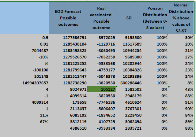
Now, if you observe the below screenshot, it is evident that one of the best possible outcomes outlaid will have a minimum error. As on 02-12-2021, its 6,364 error.

Other new measure like Poisson test will let us know if we can exactly reach 1,257,511,878 vaccinated total population today. As we can see, it is not possible and '0%' probability.

Similarly, Normal Distribution test concludes that the actual results could probably be lower than 1,257,511,878. Here, we can see mostly that, 99.1% chance that it will not increase the forecasted number and 0.9% probability that vaccines could be higher that 1,257,511,878.

The Hypergeometric distribution tells us if there is any growth on a particular day. For example Saturday! You can choose the variables as

N= Last 30 days

n= 4 Saturdays in a week

D= 1 because only once, we saw growth in vaccination from past 4 weeks

x= 1 because I only want to know if today's vaccination drive will be bustling with more number of citizens.

x=0 because I want to see if growth can be predicted or the opposite. At the moment I am in Trial & Err, and it will take 3 days for me to confirm the cumulative predictor value (0 or 1 for Growth). I will leave a message in brackets below this sentence.

All of these measures like Poisson Distribution, Normal Distribution, Monte-Carlo Simulation will increase the predictability of this model.

To speak of Monte-Carlo worksheet, it was designed to tell us if today's vaccination will be more or less than what outcome values we have chosen. I chose two and you can replace them with other outcomes from R Column. Please modify the formulas where ever needed is required for a good output.

Not the least, the Exponential Growth or Decay formula in cell R12 helped me to find out sudden spike in Indian vaccines for Saturday. For example, Saturday's formula in that cell's 'rate' variable was modified to particular day's average. That means, I averaged last 4 Saturdays daily percentage change and inserted it into the formula. This helped!

Model Analysis:

It's simple!!

You need to understand observations & their relative changes and I am sure everyone has common sense. The entire error exposure mitigation depends upon:

1. Exponential formulas

2. Averages that you choose for formulas based on past/daily observations

3. SA, SMA & EMA's average. That is, we can choose 12 days, 10 days, 5 days and 3 days average's depending upon our growth or fall interpretations/predictions from last one month or year data (Seasonal behaviour and you know it from our Pivot table).

If I find any other risk reduction techniques, I will update them as promised as it is difficult to find resources on Applied Statistics and general education does not cover research.

7 days forecast

Average percentage change in Sales/Vaccination (T1-7) = +/-99 (Last 7 days)

Last day Sales (D7) = +700 (7^th day)

Last 10 days average sales (A1-7) = 400

Alpha= 0.2

Beta= 0.17

Sort out for the above A, T and D:

1. A= 0.2(700) + (1-0.2)(400+(+99) = 140+399.2= 539.2

2. T= 0.17(539.2-400)+(1-0.17)(99)= 23.664+82.17= 105.834

3. F8= 539.2+105.834= 645.034

Now, the sales forecast for 8^th day is 645. Let us forecast for 9^th day:

1. A= 0.2(645)+(1-0.2)(645)= 129+516= 645

2. T= 0.17(645-539.2)+(1-0.17)(105.834)

3. F9= 645+ 105.83 = 750.83

Hence, the sales for 9^th day is 751.

Note that, we have to revise the model every day by updating the cells with new values i.e., Total population vaccinated collected from websites. (H2 Cell is updated daily)

Then the real data is subtracted from G2 Cell and you will get a, +/- difference. I have gathered this daily difference between Actual and Forecast numbers, stored them daily in Column V21:V43.

Step 1. Once you start forecasting, collect the difference for five days and store them in Column V.

Step 2. After 3 days, take a Simple Average of the three difference and subtract them from F8 in a separate area of the spreadsheet.

Step 3. Take the same average from Step 2 and add it to the above F8 value.

These measures will help us to reduce the error. Supposing for example, if the main difference is 100,

1. 645+100= 745

2. 645-100= 545

This will help a manager understand if he needs to produce 745 or 545 units.

Scenario 1: When sales will increase double or triple times

See here, when sales increased to 1090, our 745 estimate could not meet 345 units demand and 545 units fully sold.

Scenario 2:

Here, when the demand falls and when only 1 unit sold, 645, 545 & 745 turned into a loss. Now if we get a difference of 1000 then + or – it from 645 as usual.

Scenario 3:

Here, this method does not work because you wasted 1644 units of production and based on -355 forecast, lost sales opportunity and also produced lesser goods. This behaviour is called as Statisticians Paradox- You assumed that you have reduced the risk/error statistically based on past experiences, but the risk/error still exists (I coined this name after n observations rightfully). Hence, predicting variables is a hard job and that is one of the reason why I did not emphasize much on Least Square method of forecasting because I have to personally choose the demand.

We reduced a lot of error daily but once in a while we have this Statisticians Paradox phenomena which will make our forecast obsolete like below (common during recessions and endemics)

Surprising thing here, I only got 5 million error (G2 Cell-Actual value which I input as 73,50,000). But all the highlighted values gave a Statisticians Paradox while the model's job was to reduce the error to 1 or 2 million.

Don't feel bad if one gets an error, but learn to resolve & book mark the extraordinary. This is what all scientists did and developed their own games.

My last day file. I did it!!

22-07-2022 <-Click here

I got back to forecast again and made data changes to this hyperlinked model. I have started creating an Index for Exponential smoothing constants and included LSM Trend value forecast. It will take a week for the indexation to complete and I am anticipating that forecasts will improve. I have changed the data import to COWIN Dashboard.

23-07-2022 <- Click here

For Saturday's forecast, I have to wait until tomorrow for the real vaccinated figures to be updated. I have built the seasonal index right for Friday after I got the correct number today. So I am naturally upset about this lag in information and hence I have decided to wait for 10 days and resume forecasting and by that time, I have enough data to build complete seasonality index.

Yippeee!! After my Sunday afternoon nap which I rarely take once in a quarter, I have finished off the Seasonality index in the evening. Guess what? It is able to reduce the forecast error of Friday by 70% and Saturday's forecast error by 75%. This seasonality index is working and it's good news.

Now we've learnt 2 ways to reduce forecast errors:

a. Subtracting the forecast number from common error

b. Using the seasonality index

Seasonality index

Thus, this model is reliable for forecasting under the terms & conditions of Double exponential smoothing method.

I have two more methods that I've invented and will take a month or so. Until then...

Chao!

24-07-2022

26-07-2022

I am stopping my forecast for this month and meantime like I have advised, try it by yourself and its exciting!

28-07-2022

01-AUG-2022

26-08-2022

Hello again! I wanted to leave no tables unturned today and I have discovered more things like:

1. The seasonality index does not decrease risk as much as we had seen in our earlier model attached.

This is because there was a formula error in my last model and hence the forecast number got inflated. Due to this, the seasonality index appears to have reduced the risk. When I set all formulae straight today, the seasonality index is useful but not able to mitigate forecast error.

2. So, I went ahead and forecasted for a large data on a daily basis and the averages also don't matter or have no greater significance in reducing the risk. This is because, I have changed multiple combinations of averages to get the least error and the forecast number does not change greatly along with averages.

If you see this picture below, you will be willing to accept that counter-measure formulas have helped in achieving a forecast. That is, either of the following:

1. Single exponential formula

2. Double exponential formula

3. Exponential growth and decay formulas helped us achieve something today

See? The dark shaded forecast matches the real vaccination data. With the help of this, I was able to forecast in joy with minimum error. My errors were always in minutes and rarely in hours from below.